Youtube Streamer Analysis

Explanatory Data Analysis

Author

Data Analyst - Pythias

Published

February 6, 2024

1 OVERVIEW

This project focused on leveraging a dataset related to YouTube streamers to develop a comprehensive analysis and recommendation system using advanced data analytics techniques. The initial phase involved meticulous data cleaning to address any inconsistencies, missing values, and duplicate entries. Subsequently, trend analysis was conducted to identify patterns and fluctuations in the performance of the streamers over time. Performance metrics were calculated to gauge the effectiveness and impact of the streamers’ content. Furthermore, a content recommendation system was developed to provide personalized suggestions to users based on their preferences and viewing history. The project draws on methodologies from recommendation system tutorials, machine learning metrics, and data preprocessing for machine learning, and incorporates insights from trend analysis for business improvement. The resulting system aims to enhance user engagement and satisfaction by delivering tailored content recommendations, thereby contributing to a more enriching and personalized streaming experience.

2 DATA IMPORTATION

Code

ysa=read.csv(file.choose())

library("janitor")

ysa=clean_names(ysa)

3 DATA STRUCTURE

Code

library(dplyr)

str(ysa)

'data.frame':   1000 obs. of  9 variables:
 $ rank      : int  1 2 3 4 5 6 7 8 9 10 ...
 $ username  : chr  "tseries" "MrBeast" "CoComelon" "SETIndia" ...
 $ categories: chr  "Música y baile" "Videojuegos, Humor" "Educación" "" ...
 $ suscribers: num  2.49e+08 1.84e+08 1.65e+08 1.63e+08 1.13e+08 ...
 $ country   : chr  "India" "Estados Unidos" "Unknown" "India" ...
 $ visits    : num  8.62e+04 1.17e+08 7.00e+06 1.56e+04 3.90e+06 ...
 $ likes     : num  2700 5300000 24700 166 12400 ...
 $ comments  : num  78 18500 0 9 0 4900 0 0 32 214 ...
 $ links     : chr  "http://youtube.com/channel/UCq-Fj5jknLsUf-MWSy4_brA" "http://youtube.com/channel/UCX6OQ3DkcsbYNE6H8uQQuVA" "http://youtube.com/channel/UCbCmjCuTUZos6Inko4u57UQ" "http://youtube.com/channel/UCpEhnqL0y41EpW2TvWAHD7Q" ...

Code

ysa= ysa %>%
  rename("subscribers"=suscribers)

ysa_numeric = ysa %>%
  dplyr::select(c(rank,subscribers,visits,likes,comments))

ysa_categorial = ysa %>%
  dplyr::select(c(username,categories,country,links))

The dataset has 4 character variables and 5 numerical variables
The dataset has 1000 observations and 9 variables

Key Variables

Code

names(ysa)

[1] "rank"        "username"    "categories"  "subscribers" "country"    
[6] "visits"      "likes"       "comments"    "links"

The first 6 rows of key variable names

Code

library(knitr)
head(ysa) %>% kable()

rank	username	categories	subscribers	country	visits	likes	comments	links
1	tseries	Música y baile	249500000	India	86200	2700	78	http://youtube.com/channel/UCq-Fj5jknLsUf-MWSy4_brA
2	MrBeast	Videojuegos, Humor	183500000	Estados Unidos	117400000	5300000	18500	http://youtube.com/channel/UCX6OQ3DkcsbYNE6H8uQQuVA
3	CoComelon	Educación	165500000	Unknown	7000000	24700	0	http://youtube.com/channel/UCbCmjCuTUZos6Inko4u57UQ
4	SETIndia		162600000	India	15600	166	9	http://youtube.com/channel/UCpEhnqL0y41EpW2TvWAHD7Q
5	KidsDianaShow	Animación, Juguetes	113500000	Unknown	3900000	12400	0	http://youtube.com/channel/UCk8GzjMOrta8yxDcKfylJYw
6	PewDiePie	Películas, Videojuegos	111500000	Estados Unidos	2400000	197300	4900	http://youtube.com/channel/UC-lHJZR3Gqxm24_Vd_AJ5Yw

Summary statistics for numeric variables

Code

library(psych)
library(dplyr)
library(knitr)
ysa_numeric %>%
  summary() %>%
  kable()

rank	subscribers	visits	likes	comments
Min. : 1.0	Min. : 11700000	Min. : 0	Min. : 0	Min. : 0
1st Qu.: 250.8	1st Qu.: 13800000	1st Qu.: 31975	1st Qu.: 472	1st Qu.: 2
Median : 500.5	Median : 16750000	Median : 174450	Median : 3500	Median : 67
Mean : 500.5	Mean : 21894400	Mean : 1209446	Mean : 53633	Mean : 1289
3rd Qu.: 750.2	3rd Qu.: 23700000	3rd Qu.: 865475	3rd Qu.: 28650	3rd Qu.: 472
Max. :1000.0	Max. :249500000	Max. :117400000	Max. :5300000	Max. :154000

Summary statistics for each numeric variable

4 DATA CLEANING

Missing Values

Code

library(naniar)

invisible(ysa %>%
  gg_miss_var())

include_graphics("missing.png")

The dataset has no missing values

Duplicated entries

Code

anyDuplicated.default(ysa)

[1] 0

no duplicated entries

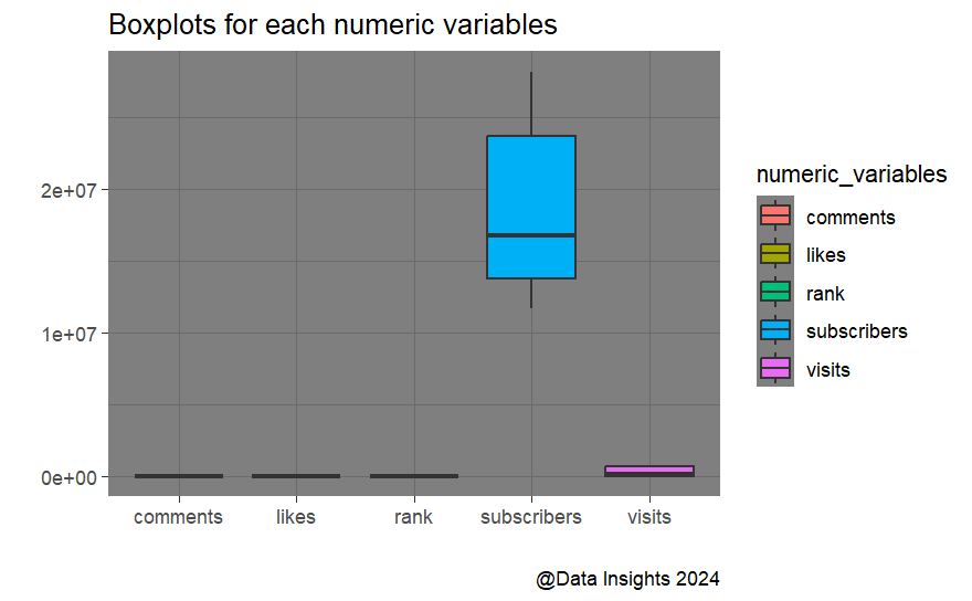
Outliers

Code

library(ggplot2)

library(tidyverse)

ysa_numeric_long = ysa_numeric %>%
  pivot_longer(everything(),
               names_to = "numeric_variables",
               values_to = "numeric_values")


invisible(ysa_numeric_long %>%
  ggplot(aes(numeric_variables,numeric_values))+
  geom_boxplot(aes(fill=numeric_variables),stat = "boxplot",position = "dodge",outlier.colour = "red")+
  facet_wrap(~ numeric_variables, scales = "free")+
  theme_dark()+labs(title = "Boxplots for each numeric variables",
                    x="",y="",caption = "@Data Insights 2024"))

include_graphics("outliers.png")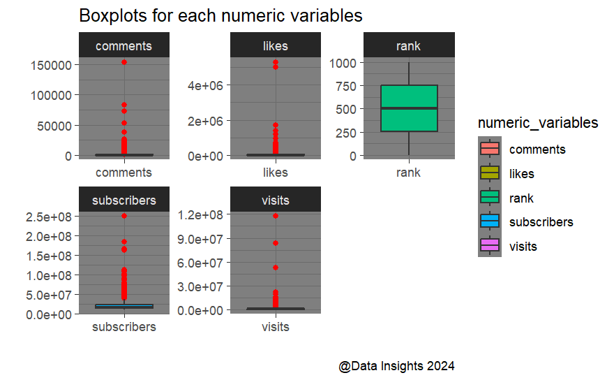

the dataset contains outliers represented by the red circles for 4 numeric variables

5 Handling outliers in the dataset

Code

library(robustHD)

ysa_numeric$subscribers=winsorize(ysa_numeric$subscribers,probs = c(0.05,0.95))
ysa_numeric$visits=winsorize(ysa_numeric$visits,probs = c(0.05,0.95))
ysa_numeric$likes=winsorize(ysa_numeric$likes,probs = c(0.05,0.95))
ysa_numeric$comments=winsorize(ysa_numeric$comments,probs = c(0.05,0.95))

#org dataset

ysa$subscribers=winsorize(ysa$subscribers,probs = c(0.05,0.95))
ysa$visits=winsorize(ysa$visits,probs = c(0.05,0.95))
ysa$likes=winsorize(ysa$likes,probs = c(0.05,0.95))
ysa$comments=winsorize(ysa$comments,probs = c(0.05,0.95))

 
ysa_numeric_long2 = ysa_numeric %>%
  pivot_longer(everything(),
               names_to = "numeric_variables",
               values_to = "numeric_values")


invisible(ysa_numeric_long2 %>%
  ggplot(aes(numeric_variables,numeric_values))+
  geom_boxplot(aes(fill=numeric_variables),stat = "boxplot",position = "dodge",outlier.colour = "blue")+
  facet_wrap(~ numeric_variables, scales = "free")+
  theme_dark()+labs(title = "Boxplots for each numeric variables",
                    x="",y="",caption = "@Data Insights 2024"))

include_graphics("outliers2.png")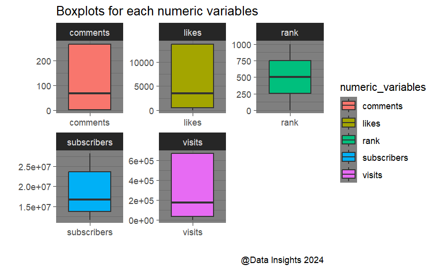

Handled outliers using robust method
As shown by the boxplots there are no longer outliers in the dataset

6 TREND ANALYSIS

Popular category

#Trends among the top YouTube streamers

Code

table(ysa$categories) %>% as.data.frame() %>%
  arrange(desc(Freq)) %>%
  kable(caption = "Most popular categories")

Most popular categories
Var1	Freq
	306
Música y baile	160
Películas, Animación	61
Música y baile, Películas	41
Vlogs diarios	37
Noticias y Política	36
Animación, Videojuegos	34
Películas, Humor	34
Animación, Juguetes	29
Animación, Humor	27
Educación	24
Películas	24
Animación	22
Videojuegos	19
Videojuegos, Humor	17
Música y baile, Animación	16
Ciencia y tecnología	14
Comida y bebida	12
Humor	10
Juguetes	10
Películas, Juguetes	9
Deportes	8
Películas, Videojuegos	8
Música y baile, Humor	6
Juguetes, Coches y vehículos	4
DIY y Life Hacks	3
Fitness, Salud y autoayuda	3
Videojuegos, Juguetes	3
Animales y mascotas	2
Coches y vehículos	2
Educación, Juguetes	2
Fitness	2
Moda	2
Animación, Humor, Juguetes	1
ASMR	1
ASMR, Comida y bebida	1
Belleza, Moda	1
Comida y bebida, Juguetes	1
Comida y bebida, Salud y autoayuda	1
Diseño/arte	1
Diseño/arte, Belleza	1
Diseño/arte, DIY y Life Hacks	1
DIY y Life Hacks, Juguetes	1
Juguetes, DIY y Life Hacks	1
Música y baile, Juguetes	1
Viajes, Espectáculos	1

Categories with unknown names are the most popular with a record of 306.
Música y baile is the second popular category with a frequency of 160.

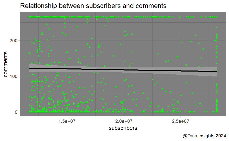
Correlation

#Correlation between the number of subscribers and the number of likes or comments

Code

sc1=ggplot(ysa,aes(subscribers,likes))+
  geom_point(color="orange",alpha=0.6,shape="circle",size=1)+
  geom_smooth(color="black",method = "lm")+labs(
    title = "Relationship between subscribers and likes",
       caption = "@Data Insights 2024")+theme_dark()

sc2=ggplot(ysa,aes(subscribers,comments))+
  geom_point(color="green",alpha=1,shape="triangle",size=1)+
  geom_smooth(color="black",alpha=1,method = "lm")+labs(
    title = "Relationship between subscribers and comments",
       caption = "@Data Insights 2024")+theme_dark()

invisible(sc1)

include_graphics("cor1.png")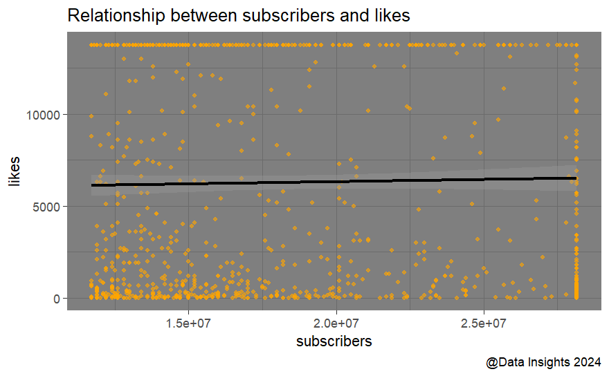

Code

invisible(sc2)

include_graphics("cor2.png")

Code

cor(ysa_numeric) %>% kable(caption = "correlations")

correlations
	rank	subscribers	visits	likes	comments
rank	1.0000000	-0.9653892	-0.0935175	-0.0266714	0.0223367
subscribers	-0.9653892	1.0000000	0.0946686	0.0232043	-0.0280959
visits	-0.0935175	0.0946686	1.0000000	0.8173862	0.6546486
likes	-0.0266714	0.0232043	0.8173862	1.0000000	0.8154030
comments	0.0223367	-0.0280959	0.6546486	0.8154030	1.0000000

Visits and likes have a strong positive relationship (r=0.82) whilst subscribers and likes have a weak positive relationship

7 AUDIENCE STUDY

Distribution of streamers audiences by country

Code

table(ysa$country) %>% as.data.frame() %>% arrange(desc(Freq)) %>%
  kable(caption = "Distribution of streamers audiences by country")

Distribution of streamers audiences by country
Var1	Freq
Estados Unidos	293
India	241
Unknown	171
Brasil	64
México	58
Indonesia	38
Rusia	25
Tailandia	18
Colombia	16
Filipinas	13
Pakistán	11
Argentina	7
Egipto	5
Arabia Saudita	4
España	4
Francia	4
Iraq	4
Turquía	4
Bangladesh	3
Japón	3
Reino Unido	3
Argelia	2
Marruecos	2
Perú	2
Ecuador	1
El Salvador	1
Jordania	1
Singapur	1
Somalia	1

Estados has the hightest number of streamers (293 audiences) followed by India with 241 audiences.
171 audiences are from unknown countries

Regional preferences for specific content categories

Code

country_categories_count=table(ysa$country,ysa$categories)
country_categories_count=as.data.frame(country_categories_count)
colnames(country_categories_count)=c("country","categories","frequency")
#sorting

country_categories_count=country_categories_count[order(-country_categories_count$frequency),]

head(country_categories_count,10) %>% kable()

	country	categories	frequency
14	India		129
11	Estados Unidos		67
881	Estados Unidos	Música y baile	53
884	India	Música y baile	42
29	Unknown		35
145	Unknown	Animación, Juguetes	28
156	Estados Unidos	Animación, Videojuegos	19
1029	India	Noticias y Política	19
899	Unknown	Música y baile	18
69	Estados Unidos	Animación, Humor	17

There are regional preferences for specific content categories such as Mysica y blue

Visual distribution of regional preferences

Code

library(plotly)

pcc=ggplot(country_categories_count,aes(country,frequency,fill=categories))+
  geom_bar(stat = "identity",show.legend = F,position = "stack")+
  theme(axis.text.x = element_text(size = 10, hjust=1,angle = 45))+
  theme(legend.position ="bottom")+labs(title = "Preferences for content categories by country")+
  theme(axis.text.x = element_text(size = 10, hjust=1,angle = 45))

ggplotly(pcc)

8 PERFORMANCE METRICS

Average number of subscribers, visits, likes, and comments

Code

colMeans(ysa_numeric) %>% as.data.frame %>%
  rename("mean"=".") %>% kable()

	mean
rank	5.005000e+02
subscribers	1.870902e+07
visits	2.935440e+05
likes	6.292061e+03
comments	1.179232e+02

Code

ysa_numeric_long2 %>%
ggplot(aes(numeric_variables,numeric_values))+
geom_boxplot(aes(fill=numeric_variables),stat = "boxplot",position = "dodge",outlier.colour = "red")+
theme_dark()+labs(title = "Boxplots for each numeric variables",
x="",y="",caption = "@Data Insights 2024")

Code

include_graphics("box.png")

Subscribers have the highest average number

9 CONTENT CATEGORIES

Code

library(knitr)

cc=table(ysa$categories)
cc1=as.data.frame(cc)
cc1=cc1[order(-cc1$Freq),]
kable(cc1)

	Var1	Freq
1		306
31	Música y baile	160
38	Películas, Animación	61
35	Música y baile, Películas	41
46	Vlogs diarios	37
36	Noticias y Política	36
6	Animación, Videojuegos	34
39	Películas, Humor	34
5	Animación, Juguetes	29
3	Animación, Humor	27
22	Educación	24
37	Películas	24
2	Animación	22
43	Videojuegos	19
44	Videojuegos, Humor	17
32	Música y baile, Animación	16
11	Ciencia y tecnología	14
13	Comida y bebida	12
26	Humor	10
27	Juguetes	10
40	Películas, Juguetes	9
16	Deportes	8
41	Películas, Videojuegos	8
33	Música y baile, Humor	6
28	Juguetes, Coches y vehículos	4
20	DIY y Life Hacks	3
25	Fitness, Salud y autoayuda	3
45	Videojuegos, Juguetes	3
7	Animales y mascotas	2
12	Coches y vehículos	2
23	Educación, Juguetes	2
24	Fitness	2
30	Moda	2
4	Animación, Humor, Juguetes	1
8	ASMR	1
9	ASMR, Comida y bebida	1
10	Belleza, Moda	1
14	Comida y bebida, Juguetes	1
15	Comida y bebida, Salud y autoayuda	1
17	Diseño/arte	1
18	Diseño/arte, Belleza	1
19	Diseño/arte, DIY y Life Hacks	1
21	DIY y Life Hacks, Juguetes	1
29	Juguetes, DIY y Life Hacks	1
34	Música y baile, Juguetes	1
42	Viajes, Espectáculos	1

Categories with highest number of streamers is unknown (306 streamers)

Categories with exceptional performance matrics

Code

cxp= ysa %>%
dplyr::select(c("categories","likes","comments","subscribers","visits"))

pe1=ggplot(ysa, aes(categories,likes))+
geom_bar(stat="identity",color="green")+
theme(axis.text.x = element_text(size = 10, hjust=1,angle = 90))

ggplotly(pe1)

In terms of likes Musica y baile has the highest number of likes

Code

pe2=ggplot(ysa, aes(categories,visits))+
geom_bar(stat="identity",color="skyblue")+
theme(axis.text.x = element_text(size = 10, hjust=1,angle = 90))

ggplotly(pe2)

In terms of visits Musica y bailee has the highest number of visits

Code

pe3=ggplot(ysa, aes(categories,comments))+
geom_bar(stat="identity",color="purple")+
theme(axis.text.x = element_text(size = 10, hjust=1,angle = 90))

ggplotly(pe3)

In terms of comments Musica y bailee has the highest number of comments

Code

pe4=ggplot(ysa, aes(categories,subscribers),color="black")+
geom_bar(stat="identity",color="orange")+
theme(axis.text.x = element_text(size = 10, hjust=1,angle = 90))

ggplotly(pe4)

In terms of subscribers, Musica y baliee has the highest number of subscribers (11 900 000 million)

10 BRANDS AND COLLABORATIONS

The dataset does not have information about that so there is a need to create a proxy variables with performance metrics

Code

ysa_numeric$brand_collaborations=ifelse(ysa_numeric$subscribers>18709023|
                                          ysa_numeric$visits>293544|
                                          ysa_numeric$likes>6292|
                                          ysa_numeric$comments>118,1,0)

brand_cor=cor(ysa_numeric)

kable(brand_cor, caption = "Correlations of perforance metrics")

Correlations of perforance metrics
	rank	subscribers	visits	likes	comments	brand_collaborations
rank	1.0000000	-0.9653892	-0.0935175	-0.0266714	0.0223367	-0.4401339
subscribers	-0.9653892	1.0000000	0.0946686	0.0232043	-0.0280959	0.4577625
visits	-0.0935175	0.0946686	1.0000000	0.8173862	0.6546486	0.5473478
likes	-0.0266714	0.0232043	0.8173862	1.0000000	0.8154030	0.5598936
comments	0.0223367	-0.0280959	0.6546486	0.8154030	1.0000000	0.5291000
brand_collaborations	-0.4401339	0.4577625	0.5473478	0.5598936	0.5291000	1.0000000

streamers with high number of performance metrics such as likes and visits are more likely to receive brand collaboration

11 BENCHMARKING

Top performing streamers in terms of likes

Code

avg_likes=round(mean(ysa$likes))
avg_visits=round(mean(ysa$visits))
avg_comments=round(mean(ysa$comments))
avg_subscribers=round(mean(ysa$subscribers))

top_streamers_likes=ysa %>%
  dplyr::filter(likes > avg_likes)

top_streamers_likes=top_streamers_likes %>%
  dplyr::select(c(username,likes))

top_streamers_likes=as.data.frame(top_streamers_likes)

top_streamers_likes=top_streamers_likes[order(-top_streamers_likes$likes),]

head(top_streamers_likes,10) %>% kable()

	username	likes
1	MrBeast	13762.56
2	CoComelon	13762.56
4	PewDiePie	13762.56
5	LikeNastyaofficial	13762.56
6	VladandNiki	13762.56
8	BLACKPINK	13762.56
9	BTS	13762.56
10	HYBELABELS	13762.56
11	ChuChuTV	13762.56
14	infobellshindirhymes	13762.56

Top 10 streamers in terms on subscribers

Code

top_streamers_subscribers=ysa %>%
  dplyr::filter(subscribers > avg_subscribers)

top_streamers_subscribers=top_streamers_subscribers %>%
  dplyr::select(c(username,subscribers))

top_streamers_subscribers=as.data.frame(top_streamers_subscribers)

top_streamers_subscribers=top_streamers_subscribers[order(-top_streamers_subscribers$subscribers),]

head(top_streamers_subscribers,10) %>% kable()

username	subscribers
tseries	28166020
MrBeast	28166020
CoComelon	28166020
SETIndia	28166020
KidsDianaShow	28166020
PewDiePie	28166020
LikeNastyaofficial	28166020
VladandNiki	28166020
zeemusiccompany	28166020
WWE	28166020

Top 10 streamers in terms on visits

Code

top_streamers_visits=ysa %>%
dplyr::filter(visits > avg_visits)

top_streamers_visits=top_streamers_visits %>%
dplyr::select(c(username,visits))

top_streamers_visits=as.data.frame(top_streamers_visits)
top_streamers_visits=top_streamers_visits[order(-top_streamers_visits$visits),]

head(top_streamers_visits,10) %>% kable()

	username	visits
2	CoComelon	665338.9
3	KidsDianaShow	665338.9
4	PewDiePie	665338.9
5	LikeNastyaofficial	665338.9
6	VladandNiki	665338.9
13	dudeperfect	665338.9
14	infobellshindirhymes	665338.9
16	TaylorSwift	665338.9
17	BillionSurpriseToys	665338.9
18	ArianaGrande	665338.9

Top 10 streamers in terms of comments

Code

top_streamers_comments=ysa %>%
  dplyr::filter(comments > avg_comments)

top_streamers_comments=top_streamers_comments %>%
  dplyr::select(c(username,comments))

top_streamers_comments=as.data.frame(top_streamers_comments)

top_streamers_comments=top_streamers_comments[order(-top_streamers_comments$comments),]

head(top_streamers_comments,10) %>% kable()

	username	comments
1	MrBeast	265.6684
2	PewDiePie	265.6684
4	BLACKPINK	265.6684
5	BTS	265.6684
6	HYBELABELS	265.6684
7	dudeperfect	265.6684
9	TaylorSwift	265.6684
10	EdSheeran	265.6684
11	ArianaGrande	265.6684
13	BillieEilish	265.6684

12 CONTENT RECOMMENDATIONS

A system for enhancing content recommendations to YouTube users based on streamers

Code

streamer_metrics <- aggregate(cbind(visits, comments, likes, subscribers) ~ categories, ysa, mean)

normalized_metrics <- scale(streamer_metrics[, -1])

library(proxy)

similarity_matrix <- proxy::simil(normalized_metrics, method = "cosine")

s=streamer_metrics$categories

user_streamer <- s # Streamers user has already interacted with

user_index <- which(streamer_metrics$categories == user_streamer)

similar_streamers <- order(similarity_matrix[user_index],decreasing = T)[-1]

recommended_streamers <- streamer_metrics$categories[similar_streamers[-1]] # Exclude the user's own streamer

recommended_streamers %>% as.data.frame %>% 
  rename("Recomended Categories for enhancing content"=".") %>% kable()

Recomended Categories for enhancing content
Música y baile
Videojuegos, Humor
Noticias y Política
Moda
Películas, Videojuegos
Música y baile, Juguetes
Películas, Humor
Educación
Películas
Comida y bebida, Juguetes
Películas, Juguetes

Deportes
Música y baile, Humor
Música y baile, Películas
DIY y Life Hacks, Juguetes
Juguetes
Educación, Juguetes
Diseño/arte, Belleza
Animación, Humor
ASMR, Comida y bebida
Comida y bebida
Juguetes, Coches y vehículos
Diseño/arte, DIY y Life Hacks
Animación
Videojuegos, Juguetes
Videojuegos
DIY y Life Hacks
Música y baile, Animación
Viajes, Espectáculos
Animación, Juguetes
Comida y bebida, Salud y autoayuda
Películas, Animación
Fitness
Animales y mascotas
Diseño/arte
Animación, Videojuegos
Juguetes, DIY y Life Hacks
Belleza, Moda
Coches y vehículos
Fitness, Salud y autoayuda
ASMR
Vlogs diarios
Ciencia y tecnología

The recommended youtube streamers belong to those categories.
These categories help to classify streamers and provide a basis for recommending content to users with similar interests.

13 KEY FINDINGS

Animacon is the most popular category with 306 streamers.
Number of visits and likes have a string positive relationship.
Estados Unidos is the country with the highest number of 293 streamers, followed by India with 241 streamers.
Moda category has an exceptional performance metrics of more than 500 000 likes, 25 000 000 visits, more than 15 000 comments and 3 000 000 000 subscribers.
Top 10 streamers have an average number of 13762 likes, 281 666 020 subscribers, 665338 visits and 205 comments